

Machine Learning
Working with Unbalanced Distributed Data - Oversampling Method
What should we pay attention to when modeling on an unevenly distributed data set? If we do not have enough data for the label we are estimating, what methods should we apply? If the importance of the labels is not the same, how should we create our model? Let's find out the answers to these questions together. While working with a sample dataset, we will look for answers to these questions and examine the methods used in detail.
In this study, we will work with the data containing fraud data on the credit card. The most important feature of this dataset is that the data is not distributed properly to the labels. The number of non-Fraud data is 284315. The fraud data number is 492. There is a very big difference. Although the number of fraudulent data in our data is very small, the importance of this label is much more important for us than the other label. Catching fraud transactions is our priority in such studies. The number of data is small, the level of importance is high, and we should focus more on this label. How do we do that? Let's start our project and look for answers to these questions.
data = pd.read_csv('creditcard.csv')
Let's check if there is any missing data in our data.
data.isnull().sum()
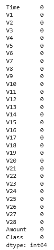
There are no missing data in our data set. Very nice! Let's continue our study by looking at the distribution of labels.
data['Class'].value_counts()
0:  284315
1:    492

There is a huge imbalance in the distribution of data. When we get to the modeling stage, we will try to get rid of this data imbalance. Before reaching this stage, we separate our data into train, test and valid data. We will train our model on train data. Our validation data will allow us to analyze the state of the model while the training process is ongoing. The test data will not be seen by our model until the end of the training. We will use this data during the evaluation phase of the result of our model. Let's divide our data into three.
from sklearn.model_selection import train_test_split
X_train, X_test, y_train, y_test = train_test_split(X, y,
                                  test_size=0.25, random_state=42, stratify=y)
X_test, X_valid, y_test, y_valid = train_test_split(X_test, y_test,
                                  test_size= 0.70, random_state=42, stratify=y_test)
The next stage is the standardization of our data. By standardizing the data, we will ensure that the data is converted into a standard form. As a result of this process, our model will be able to evaluate the data more accurately and impartially. At the same time, our model will run faster because the size of our data will also decrease. At this stage, we will use the StandardScaler method.
from sklearn.preprocessing import StandardScaler
scaler= StandardScaler()
X_train = scaler.fit_transform(X_train)
X_test = scaler.transform(X_test)
X_valid = scaler.transform(X_valid)
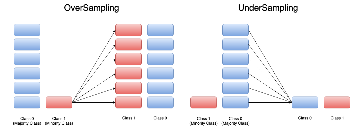
We have standardized our data with the above code. At this stage, we will try to solve the problem of data imbalance. We will apply oversampling method on our data.
What is Oversampling Method, What Does Oversampling Do?
Oversampling is a method that allows us to intervene in the distribution of data when the distribution of data is irregular. We equalize the number of data in labels by randomly multiplying the data of the label that has less data than the other. Subsampling, on the other hand, is a method of randomly reducing the data of a label that has more data than others. The goal here is to equalize the number of data in labels in the same way. We will use the oversampling method in our project.
Let's examine together how this process will be implemented.
from imblearn.over_sampling import RandomOverSampler
oversample = RandomOverSampler(sampling_strategy='minority')
X_train, y_train = oversample.fit_resample(X_train, y_train)
We can do this very easily by using the RandomOversample class. We ensure that the data is increased according to the label with the least data. we can make this adjustment easily with the "sampling_strategy" parameter. At the next stage, we start increasing the data with the "fit_resample" method. The important point here is that we are doing this operation only on train data. Our goal is to eliminate the imbalance in the educational stage. We do not apply this process for validation and test data. This data should stand in its initial form, as it should be. In this way, our results will be more reliable. Let's look at the latest situation in our train data
y_train.value_counts()

0    213236
1    213236
As can be seen above, as a result of the process we have implemented, we have ensured that the number of data on the labels in the training data is the same.
We have cleaned up the data, standardized it and organized the amounts of data. The data preprocessing phase ends here. Our next stage is the modeling stage. Let's see what we're going to do together.
Creating Model with Unbalanced Distributed Data
At this stage, we will use several different modeling algorithms. Although we equalize the number of data for labels, we may not get enough efficiency from the model. For this reason, there will also be points that we will pay attention to during the modeling phase. At this stage, we will use multiple models (ensemble learning) together instead of a single model.
What is the Ensemble Learning Method?
The method by which multiple models make predictions together in an integrated manner is the ensemble method. This method allows us to combine the strengths of the models. This approach is a frequently used method in cases where the data distribution is not inequel. In addition, the ensemble method can prevent the occurrence of excessive learning problems and ensure that the results are more stable. There are different types of ensemble method. We will use a less complex ensemble method in our project. We will train the models separately and combine the predictions of these models. As this method could be used, the models could also be trained together. This is a situation that may vary depending on the data and the project.
During the modeling phase, we will use Logistic Regression, XGBOOST, KNN (K Nearest Neighbors) models separately and combine the results of the models.
What is Logistic Regression?
Logistic regression is a successful algorithm that is used very often in binary classification. The algorithm uses the sigmoid function at the calculation stage. Using this function, we obtain a probability value as to which class the data belongs to as a result of the operation. We can classify our data using these probability values. In the following image, you can examine how logistics and linear regression approach the data.

We can easily do this process in python with the following code.
# Model
lr = LogisticRegression(penalty='l2', class_weight = {1:4,0:1}, C=0.001 , max_iter=200)
lr.fit(X_train, y_train)
lr_pred = lr.predict(X_test)

#Results
recall:  0.9302325581395349
precision:  0.01773049645390071
accuracy:  0.9109568427599767
f1-score:  0.034797738147020446
The class_weight parameter is important here. With this parameter, we enable the model to learn these data better by stating that the data with the label "1" (fraud) is more important. We set up our model, train it, and then we get the above results. Our model correctly estimates 93% of the data with the "1" label. We were able to access this information with the Recall metric.
The other algorithm we use in our project is the KNN algorithm.
What is KNN Algorithm (K Nearest Neighbors Algorithm)?
The KNN algorithm is an algorithm that examines and evaluates which class the data closest to the data is included in before classifying the data. As a result of this review, it decides which class the newly received data will be included in. It is an important situation how many neighbors will be looked at during this examination stage. The number of neighbors to be examined should be adjusted accordingly to the data.
Let's explore together how to do it with Python.
# Model
from sklearn.neighbors import KNeighborsClassifier
knn = KNeighborsClassifier(n_neighbors=5,
                           weights = "distance")
knn.fit(X_train, y_train)
y_pred = knn.predict(X_test)

#Sonuçlar

recall:  0.813953488372093
precision:  0.7291666666666666
accuracy:  0.9991573202784856
f1-score:  0.7692307692307692
Our model examines the 5 closest neighbors. We also gave the "distance" value to the "weight" parameter. In this way, we ensured that the weight of the distant data was less and the weight of the nearby data was more during the learning and forecasting stages. Our recall value is lower compared to the previous model. Although our model is not as successful as the first model in predicting fraud data, it still has a rate that can be considered good. In addition, our model is quite successful in predicting the "0" label.
The last algorithm we use is the XGBOOST algorithm.
What is XGBOOST Algorithm?
The XGBOOST algorithm is a tree-based algorithm. The algorithm uses multiple trees while classifying the data and makes the prediction according to the common decision. Because of this feature, the XGBOOST algorithm is also an example of the ensemble model.
We can use this algorithm with the help of the following code.
import xgboost as xgb

# Model

dtrain = xgb.DMatrix(X_train, label=y_train)
dtest = xgb.DMatrix(X_test, label=y_test)
dvalid = xgb.DMatrix(X_valid, label=y_valid)
params = {
    "objective": "binary:logistic",
    "eval_metric": ['error', 'logloss'],
    'n_estimators':2000,
    "max_depth":2,
    "eta": 0.1,
    "gamma": 1,
    "subsample": 0.8,
    "colsample_bytree": 0.8,
    "seed": 1,
    "scale_pos_weight" : 10
}
model = xgb.train(
    params=params,
    dtrain=dtrain,
    num_boost_round=100,
    early_stopping_rounds=5,
    evals=[(dvalid, "Valid")],
    verbose_eval=5)


#Results
recall:  0.9302325581395349
precision:  0.02075765438505449
accuracy:  0.9241588250637026
f1-score:  0.04060913705583756
The parameter "eta" represents the learning rate. With this parameter, we determine at what rate the model will update itself with the newly learned data. We determined the importance level of the tags with the "scale_pos_weight" parameter. we have stated that the "1" label is more important. We used our validation data in this model. Our model will develop itself in a cycle for a certain period of time. At this stage, it will check the amount of errors in the validation data and terminate the training process if there is no improvement. When we look at the results, it is seen that our recall value is better than the value in the KNN algorithm. Our accuracy value is higher than our accuracy value in logistic regression. We have achieved a balanced result with the XGBOOST model. We will take advantage of this situation at the stage of combining the results of the models.
Let's combine the results!
The process we will do at this stage is very simple. We will take the average of the probability values. How so? First of all, let's look at a simple example.
| Model | Probability |
| Model - 1 | 0.60 |
| Model - 2 | 0.45 |
| Model - 3 | 0.15 |
Let our models and the probabilities they predict be as above. What will be the result?
The result will be shaped as (0.60 + 0. 45 + 0.15)/3 = 0.40 . We collected the probabilities and calculated their average.
Of course, we may not want all 3 models to affect the result equally. In this case, we can change the weight of the models by multiplying the results obtained by coefficients. In our project, the models will not affect the result equally. The XGBOOST algorithm, which gives a more balanced and stable result, will have a greater impact on the result than other algorithms.
import numpy as np
# XGBoost
xgb_preds = model.predict(dtest)

# Logistic Regression
lr_preds = lr.predict_proba(X_test)[:, 1]

#knn
y_pred_knn = knn.predict_proba(X_test)[:, 1]

#Ensemble
katsayılar = [3,1,1]
ensemble_preds = np.sum([katsayılar[0] * xgb_preds,
                 katsayılar[1] * lr_preds,
                 katsayılar[2] * y_pred_knn], axis=0)/sum(katsayılar)
We combined the results of our models with the code above. We have adjusted the weight of our XGBOOST model to be 3 times that of other models. Let's look at our latest rates.
Ensemble recall:       % 93.02325581395348
Ensemble precision:    % 3.5056967572304996
Ensemble accuracy:     % 95.56991232118136
Ensemble f1-score:     % 6.756756756756757
We ensured that the recall rate remained at 93%. Although we could not improve this ratio, the fact that we were able to maintain it is enough for us. While keeping the recall value at a certain level, we were able to increase the accuracy rate thanks to the ensemble method. Let's also examine how our estimates are distributed on the confusion matrix.
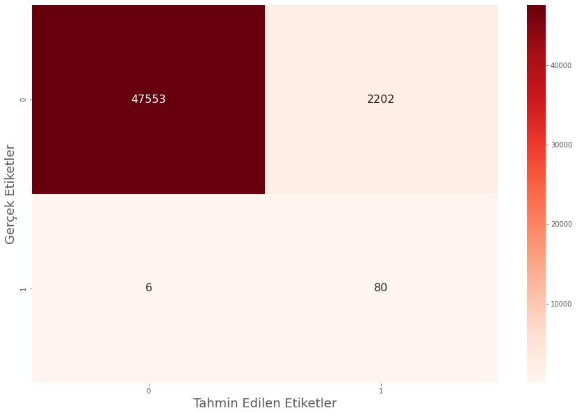
We guessed correctly 80 out of 86 fraud data. At this stage, we classified 2202 non-fraud data as fraud and made a wrong guess. Although this number seems like a lot, the result is successful considering the disproportionate distribution of the labels, the scarcity of data in the "1" label and the importance of the "1" label.
If you want to contact me or follow up;
Linkedin: www.linkedin.com/in/mustafa-bayhan-410a2a226/
Kaggle : www.kaggle.com/mustafabayhan
Data set and Code:
Data set: www.kaggle.com/datasets/mlg-ulb/creditcardfraud
Code : www.kaggle.com/code/mustafabayhan/
About author

Mustafa Bayhan
Hi, I'm Mustafa Bayhan. I am an Industrial engineer who works in data-related fields such as data analysis, data visualization, reporting and financial analysis. I am working on the analysis and management of data. My dominance over data allows me to develop projects in different sectors. I like to constantly improve myself and share what I have learned. It always makes me happy to meet new ideas and put these ideas into practice. You can visit my about me page for detailed information about me.
You may also like

0 Comments
Leave a Reply
Recent Posts

Kumru AI İncelemesi: Güçlü Yönleri, Zayıf Yönleri ve Kullanım Deneyimi

Large Language Models (LLMs): RAG, Context Engineering, and AI Agents

Model Selection in Data Analysis: What are AIC and BIC?

Types and Meanings of Histograms Used in Data Analysis

Can Correlation Be Used to Infer Causality?

Histogram Nedir, Histogram Grafiği Nasıl Yapılır?