What is Vlookup in Excel, How to Use Vlookup in Excel?

Have you ever searched for data in excel and couldn't find it? How boring does it sound to get lost in hundreds of data and waste time? We will examine a very important excel formula that will do the search for us: Excel VLOOKUP Formula. With  VLOOKUP formula, which is a very useful formula that we use in many projects, we can both speed up projects and prevent possible errors. If your path has also fallen into Excel and you wondered what is  VLOOKUP formula, you are in the right place. Let's look for answers to the questions of what is VLOOKUP formula and where is VLOOKUP formula used!

What is VLOOKUP in Excel?

VLOOKUP formula is the most important excel formula that is frequently used when looking for results that correspond to specific values in a data set. By using VLOOKUP formula, we can filter the data according to certain characteristics in excel and easily achieve the desired results.

How to Use VLOOKUP in Excel? 

The general structure of the VLOOKUP formula is shown below. Let's examine the parameters here together.

=VLOOKUP(lookup_value, table_array, col_index_num, range_lookup) 

lookup_value: This parameter specifies the value to search for. The value we are looking for in the data set is written here. There is a very important point to be considered here. In which column will this data be searched? This data is searched in the first column in the field we select. In the next parameter we will select a range on the table. When doing this process, care should be taken that the column of the value to be searched is at the beginning. This is a big disadvantage for this function. We will discuss this disadvantage below.

table_array: This parameter selects a field where we will search for data. The first column of this selected field must be the column we are searching for and this selected field must contain the result column.

col_index_num: With this parameter, we specify which column is the result column in the selected field.

range_lookup: This parameter takes a value of 0 (FALSE) or 1(TRUE). If we give the value 0, we indicate that we only want results that match exactly. On the contrary, in the opposite case, we state that we do not want a hundred percent match. When this parameter gets the value of 1, the Vlookup formula will also bring values close to the result we are looking for. If this parameter is set to 1, the values in the first column should be ordered (the column should be ordered from A to Z in textual data and from small to large in numerical data).

What can be done with VLOOKUP Excel Formula?

1) Let's imagine that we want to access the personal information of the staff in a large file, we need to find out the responsibilities of the employees in the project, or we need to know how long an employee has been absent from work. Many similar situations occur very often in business life and take a lot of time. The vertical formula will be able to successfully perform all these tasks and save time.

2) With VLOOKUP function, we can easily access the stock status, price and feature of the products.

3) With VLOOKUP formula, we can control the products our customers buy, the payments they pay and how often they shop.

These situations are just examples for the use of VLOOKUP in excel. VLOOKUP formula will work successfully in many projects similar to these examples.

Excel Vlookup Example Study

Let's make an vlookup example to better understand both the above parameters and the use of excel vlookup formula. We will search for the values in the table with vlookup formula and use the matching data. Let's do it then!

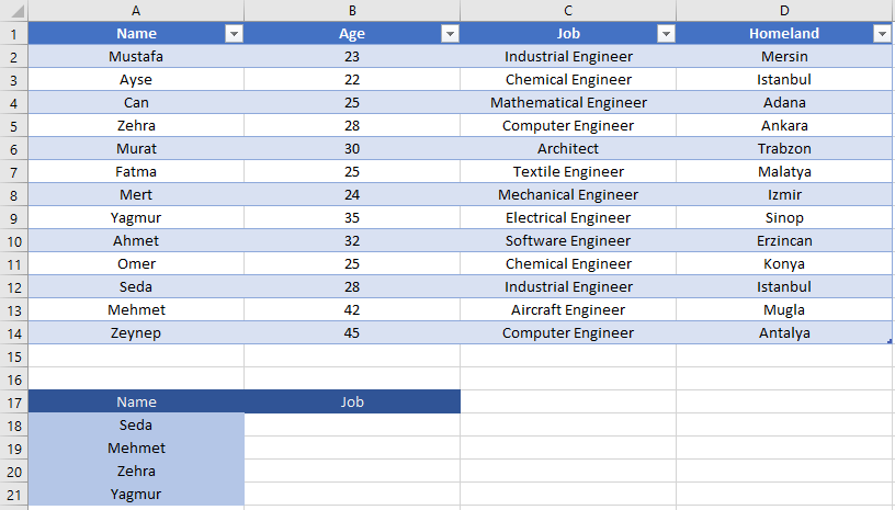
Suppose we have the above data and we are looking for the occupation of the bottom 4 people. What are we going to do in this situation? First, we will search for these names in the first column in order. When we find the data we are looking for, we will reach the profession that corresponds to this name. Here is the function that allows us to do this operation, the VLOOKUP formula.

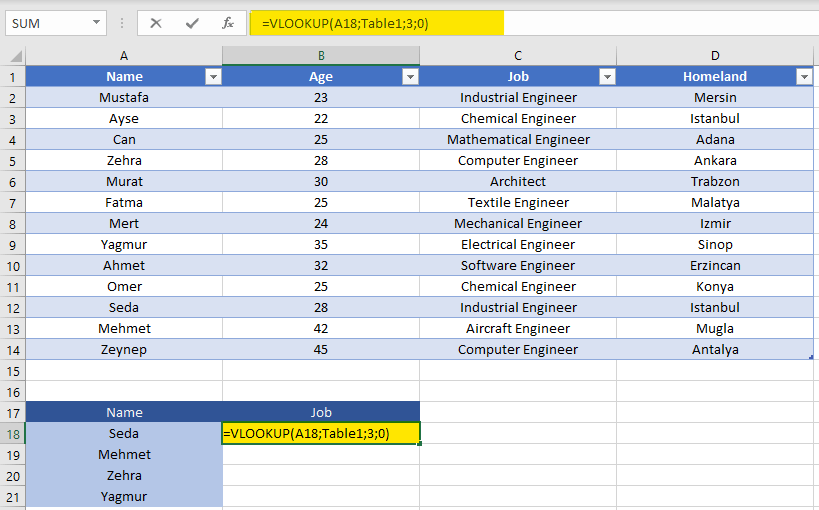
We have written VLOOKUP function above, starting with the equal to the empty cell. We selected cell A18 as the first parameter. This means that we will search for the Seda data written in A18 in the first column of the table we have selected. The second parameter represents the section we have selected in the table. It tells us that we have chosen Table1. Already in the picture, the selected part of the table appears in color. The third parameter is the order of the target column. We are looking for professions and the profession column is the 3rd in the range we selected. since it is a column, we give the value 3 to this parameter. As the last parameter, we also specify that we want an exact match (we wrote 0). Let's see the result.

VLOOKUP Formula searched for the name Seda in the first column and printed the occupation data in the row it found in the cell. Our first search was very successful, but will we write vlookup formula all the time for other cells? Of course not! The excellent side of Excel is revealed here.

As seen above, when we select the cell, a dot appears in the corner. When we click on this point twice, the function will be copied down automatically and we will have reached the desired values. Let's see the result.

The cell numbers in the formula were also automatically updated while the function was copied to the cells below. Although we searched for Seda in the first operation, the value searched for slipped downwards as the function slid downwards and the Mehmet, Zehra and Yagmur values were searched respectively. This is the general use of VLOOKUP in excel.

How to Get Rid of the Error #N/A Excel?

What will happen if the expression we are looking for with VLOOKUP formula is not in the range? In this case, VLOOKUP formula gives the #N/A error. Although this is a very usual result, it is dysfunctional in many studies. For example, if we are looking for a value consisting of numbers and we are going to mathematically sum the results we find, #N/A error will disrupt our work. So what can we do when we get a #N/A error? We can avoid the #N/A error by using the IFERROR formula. By using the structure below, we can easily integrate these two formulas.

=IFERROR(VLOOKUP(), process)

When we use VLOOKUP function in this way, we can easily solve the #N/A error. For example, we can write the value 0 in the process parameters. If the formula does not find a value in the search result, it will return the value 0 instead of the #N/A error.

What are the Disadvantages of Excel VLOOKUP Formula?

Excel VLOOKUP formula has two main problems. The first problem of the VLOOKUP formula is that it searches the data line by line in excel. This prolongs the process when working with large data and causes loss of time. The second problem of VLOOKUP formula is that the column to be searched must be at the top when searching data in excel. For this reason, our target column must be located to the right of the value searched column. When searching with Vlookup, we can search towards the right columns. If there is a column to the left of the lookup column and we are trying to access the data here, unfortunately we will not succeed

If you want to be informed about the developments and case studies about statistics, excel and excel formulas, you can follow me from the accounts below.

Linkedin: www.linkedin.com/in/mustafabayhan/

Medium: medium.com/@bayhanmustafa

Additionally, you can sign up for the newsletter via the link below and easily follow the articles in this area.

Subscribe to Newsletter

If you can read it until the end without getting bored, this applause is for you.