

Data Science
What is Time Series Analysis? What is time series forecasting?
Would you like to know the future price of the products you want to buy? So, would it benefit you to know the future value of the shares you will invest in? It would be nice if you knew how much your company will sell next year, wouldn't it? So, what would you think if I told you that all this can be done? Here's the secret formula: Time travel, of course not. The mysterious formula that allows us to do this and much more is time series analysis. Let's examine the time series together!
What is Time Series?
Time series are sorted by time; they are a set of interrelated data affected by change of time. The value of a data in a series is shaped according to the data before it and the change of time. The most common mistake made in time series analysis studies is the idea that every data categorized by time is a time series. For example, a dataset containing the number of surveys conducted by day is not a time series. Data like this move independently of each other and time. For this reason, this and similar data are not used in time series analysis.. When performing the time series analysis, it should be noted whether the data is suitable for the analysis. So what are the situations that make up the time series? Let's examine the appropriate time series situations with a few examples.
Time Series Data Examples
• Changes in the values of stocks over time
• The change in the price of a product over time
• Weather data
• Sales data
• Stock Market Price
are examples of a time series.
What is a time series forecast?
Time series prediction is the process of predicting future data with the help of previous data. At this prediction stage, the historical data are changed and edited by applying various operations. Thanks to the operations applied to the data, our projects will become easier at the stage of predicting future data and our results will be much better. The most important of these operations are the adjustments applied to the data. The suitability of the adjustment used in the analysis to the data has a significant impact on the outcome of the analysis. We will examine the types of adjustment and how these adjustment are applied to the data in detail in the later stages of our article.
So why are we making predictions with time series data? To be able to make our plans more realistic, to get an advantage while achieving our goals and, of course, to earn a little money. Let's take a closer look and learn the methods of time series analysis.
What are the Time Series Data Components?
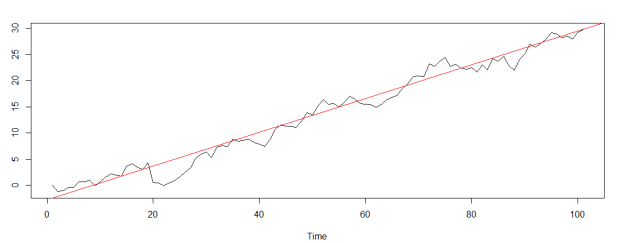
1) What is the Trend Component in Time Series Data?
The trend component represents the overall tendency that the data in the series shows in a certain direction over a certain time period. In other words, the trend component is an indicator of which way and in which direction the data is moving over a certain time period. The following shows a time series and the general pattern (trend) of the data.
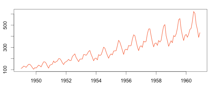
2) What is Seasonality Component in Time Series Data?
Seasonality is the effect of time change on data. The data may show similar characteristics with the same period of the previous years at certain periods of the year. For example, the consumption of cold drinks increases in summer and decreases in winter. This data shows similar behaviors in the same period of each year. This is known as the seasonality effect.
3) What is The Cyclical Component in Time Series Data?
The cyclical component is the situations that occur depending on a certain event or decision and affect the data in the long term. These cycles, which can last for more than a year, usually occur as a result of changes in the business world, economic policies and political decisions. The cycle of prosperity, recession, depression and recovery, known as the business cycle, is a good example of the cyclical component.
4) What is the Noise in the Time Series Model?
There are many external factors that affect the data, and the effects of these factors on the data are usually irregular. All of the external effects that cannot be explained by the model, and it is unknown exactly when and how much they will affect the data, are called the noise. The Noise is the result of unforeseen events such as earthquakes, wars, pandemics. Irregularity in the data (Noise) is an important factor that directly affects the result of the analysis. In order to increase the success of our analysis, the amount of noise in the data should be reduced. In order to reduce the noise in the data, Smoothing Techniques are often used. We will examine these techniques in detail in the continuation of our article. Let's examine together what is the concept of Stationarity, which has a very important place in the time series.
What is Stationarity in Time Series Data?
Stationarity is that the statistical values of the data do not change in a certain time period. The data we reviewed may vary within this range. The important point is that the mean, variance and covariance values of the data in this period do not change. If these conditions are met, the data is stationary in this time period. We can examine whether our data is stationary with the help of Dickey-Fuller and Phillips-Perron tests.

Before starting the analysis, we should perform a stationarity test for the data. If our data is not stationary, we should make our data stationary. So how do we stabilize our data? Let's examine it together!
What is the Method of Differencing in Time Series Model?
The method of differencing is a technique that is applied when the data is not stationary and allows to make the data stationary. In this simple but frequently preferred method, the previous data is extracted from each data in the series. Thanks to this process, a new series is obtained. It is not certain that this new series is also stationary, and a stationary test should also be performed for the new series. If the data has been made stationary, the analysis is continued with this new data.
After this stage, we will examine what we can do to reduce the noise in the data and what correction techniques work.
What are Smoothing Techniques in Time Series, Where Is Smoothing Used?
Smoothing is a method that allows us to remove noise from the data. With this method, we soften the changes that the model cannot explain in the data and make the meaningful parts of the data more obvious. Let's take a look at a few commonly used correction techniques together.
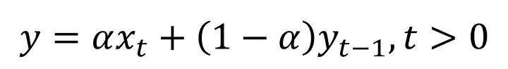
1) What Is Single Exponential Smoothing in Time Series?
Simple exponential smoothing is a smoothing method used when there is no trend and seasonal effect on the data. This smoothing technique usually performs better on stationary data. Let's examine how we use this method!
If the formula scares you, you can calm down. We have not yet reached the stage where we should be afraid : )
Although it sounds complicated, the formula adopts a simple principle. When creating a new forecast, we use the real value of the data we process and the smoothed version of our previous data. So which of these two numbers do we have to pay more attention to? We make this arrangement with the alpha parameter. By giving this parameter a value in the range of 0-1, we are adjusting the coefficients of the two data that we use when estimating for new data. Thanks to this process, we determine which of the two data we will use at what rate when creating our new data. More confused isn't it :) Let's examine it by making an example!
Let's assume that the 5th value in our series is 100 and its smoothed version is 80. Let's set the value of 0.3 as the alpha parameter. Let's calculate the smoothed version of the 6th data in our series.
Y6 = 0.3 * 100 + (1 - 0.3) * 80 = 86
In the formula, we did not do anything other than write our values in place. As a result, we calculated the real value of our 6th data as 100 and the smoothed value as 86. We apply this process for all data in the series and we will soften our series. In this example, we set the coefficient of the smoothed value in the previous iteration larger and increased its effect on the result.
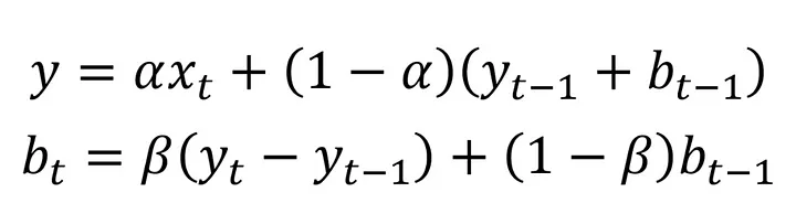
2) What Is Double Exponential Smoothing in Time Series?
The double exponential smoothing method is a smoothing technique that is generally used when there is a trend effect in the data. In this correction method, we use the data from the previous stage while creating the smoothed version of our data. There are two equations in this method, which is a bit more complicated. With the help of the first equation, we perform the smoothing operations on our data. The second equation allows us to include the trend effect in the smoothing process. In these two equations, we use parameters named alpha and beta. These parameters can take values in the range of 0 - 1. With the help of these parameters, we can adjust which data we will use when creating a new forecast. We will understand better with an example. Let's make an example!
| Stage | Actual X | Smoothed X | b (trend) |
Alfa value |
Beta value |
| 5th stage | 10 | 12 | 4 | 0.3 | 0.4 |
| 6th stage | 15 | ? | ? | 0.3 | 0.4 |
Let's calculate the smoothed version of our data in the 6th stage and our new trend value using the values from the 5th stage.
y = 0.3 * 15 + (1 - 0.3) * (12 + 4) = 15.7
The actual value of the 6th data in the series was 15 and we were trying to find the smoothed version of this data. With the above process, we calculated the smoothed version of our data as 15,7. So where did we use the trend? Our trend value (b) in the previous stage was 4. By substituting this value in the equation, we have added the trend effect to the new forecast. Is it over? Of course not. Next we have the operations for our trend equation. We will update our "b" value and make our trend value ready for use in the next step. Let 's do it!
b (trend) = 0.4 * (15.7 - 12) + (1 - 0.4) * 4 = 3.88
The old value of the trend was 4 and the updated value was 3.88. Our new trend value is ready for use in the next phase.
We continue by applying the operations in these two equations for each data and we will smooth all the data in the series.
You thought it was over, didn't you? Hold on tight, we're just getting started.
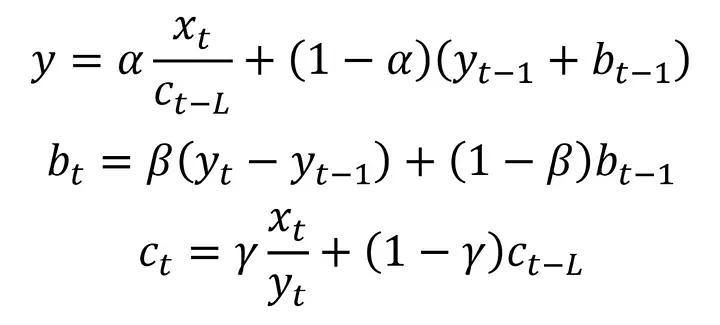
3) What is Triple Exponantial Smoothing in Time Series?
Triple exponential smoothing, also known as Holt-Winters' exponential smoothing, is a method used in time series with seasonality effect and allows to integrate seasonality into forecasts. Although this method, with the equations below, may seem very complicated, it basically has similar features to other methods. In addition to this method, there is a third equation representing the seasonality effect. There is also a parameter (alpha beta and gamma) for each component (equation). With these parameters, we determine to what extent the data we use while creating our estimation will affect our estimation. The trend equation (2nd equation) in the method is the same as the trend equation in the double exponential correction. The only difference in the first equation is that we divide the actual value of our data by the seasonality value (c). Thanks to this process, we remove the seasonality in the series from the data. Seasonality was when the data exhibited similar behavior over certain time periods. For this reason, when updating the seasonality value, the seasonality value from a certain time ago is used. The length of this period varies according to the seasonality in the data and is represented by the symbol L in the formula below. Let's continue with an example.
| Stage | Actual X | Smoothed X | b | c |
Alpha |
Beta | Gamma | L |
| 5th stage | 10 | 12 | 4 | 3 | 0.3 | 0.4 | 0.2 | 2 |
| 6th stage | 15 | ? | ? | ? | 0.3 | 0.4 | 0.2 | 2 |
Let's find our new b (trend), c (seasonality) and smoothed x values in step 6 by substituting the values in the table into the equations. Let's start with our first equation.
For seasonality, we set the period length (L) as 2. For this reason, we will use the seasonality value 2 stages ago when making the operations. We need the seasonality value in the 4th stage when performing the operations in the 6th stage. Suppose this value is 1.2.
c4 = 1.2
y = 0.3 * (15 / 1.2) + (1 - 0.3) * (12 + 4) = 14.95
The value of our 6th data was 15. As a result of the smoothing process, our data turned into 14.95. Let's continue by updating our trend and seasonality values to use in the next stages.
b = 0.4 * (15.7 - 12) + (1 - 0.4) * 4 = 3.58
Our trend value (b) in the previous stage was 4. We calculated our updated trend value as 3.58. In this way, we have prepared our trend value that we will use in the next step. We will use 3.58 instead of 4 when calculating the smoothed value of the 7th data. Great, now let's update our seasonality value.
c6 = 0.2 * (15 / 14.95) + (1 - 0.2) * 1.2 = 1.16
Using the seasonality (c) value in the 4 stages, we found the c value in the 6th stage to be 1.16. Since our period length is 2 units, we will use this calculated value when processing the 8th data.
By doing these operations for each data in the series, we smooth all the data and remove the noise in the time series from the series.
Something must have caught your attention in our operations so far. As it is noticed, we smooth our data and update our values by using the previous data at every stage. So, how do we smooth out our first data? When smoothing the first data, we usually set the initial points ourselves and start the process in this way. The initial point we set are also an important factor that affects the result of our analysis. For this reason, care must be taken when determining the initial value.
How to forecast in time series analysis?
Before proceeding to the estimation phase, a stationarity test should be performed for the data and if there is a lot of noise in the series, appropriate smoothing processes should be applied. We have examined these processes in detail above. The next step is the estimation phase. We will examine the data prior to the data we are trying to predict using certain techniques. We will try to predict future data in the light of these reviews. So how many prior data will we examine when trying to predict future data? This is a situation that varies according to the data. The number of how many data will be examined is called lags. For example, if we are trying to estimate the 7th data and our lag value is 2, we will use our 6th and 5th data in the estimation phase. If our lag value was 3, we would examine data 4, 5 and 6 while estimating data 7. Let's continue by examining the estimation techniques!
What are the time series estimation methods?
Statistical methods such as Auto Regression (AR), Moving Average (MA), ARMA, ARIMA, SARIMA, VAR and VARMA, and machine learning techniques such as artificial neural networks and LSTM are the methods frequently used in time series estimations. Each of these methods is an important area that needs to be studied in detail. The suitability of the method used with the data and the establishment of the model with the correct parameters are important factors affecting the result of the analysis. So how do we decide on the right model and the right parameter values? Two of the most frequently used methods when deciding on the model and its parameters are the ACF and PACF methods. Let's examine these methods together.
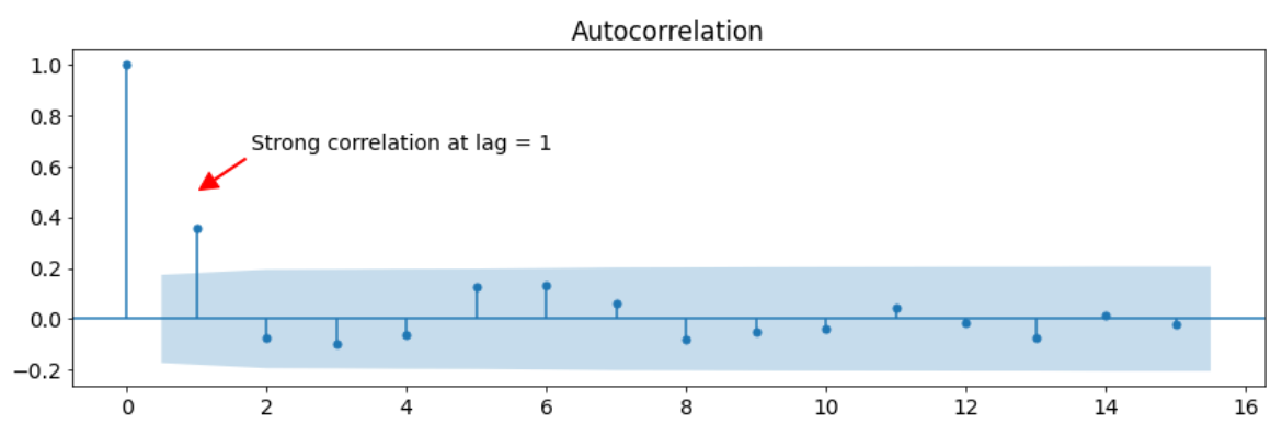
What is ACF Method and Where Is It Used?
ACF (Autocorrelation Function) is a type of graph that shows autocorrelation in data according to delay values. Correlation is a term that shows the relationship between two data and takes values between -1 and 1. The closer the correlation value is to 1, the greater the positive correlation between the data. On the contrary, when our value approaches -1, the negative relationship between our data becomes stronger. In the ACF method, a graph is created according to this principle. The ACF chart shows the correlation of the current data with historical data. For example, when we examine the ACF graph below, it is seen that the current data has approximately 0.4 correlation with the 1 data before it. Likewise, the current data has a correlation of approximately 0.2 with the previous 6 data. While determining the lag number, we examine the correlation values in this graph and the direction of the relationship.
What is the PACF Method and Where Is It Used?
The PACF method is a method that shows the ratio of direct relationships by ignoring the indirect relationships in the data. So what is a direct relationship and an indirect relationship? An indirect relationship is that the data are linked to each other through other variables. For example, ice cream sales and slipper sales increase in summer, but decrease in winter. Although these two data act similarly, they are indirectly related to each other, not directly. The reason for this is that a third variable, the temperature variable, connects these two data. These data are not affected by each other but by the temperature variable. This relationship is an indirect relationship. A direct relationship is the situation in which data directly affect each other. If we examine it through the same example, temperature and ice cream sales have a direct relationship. The change in temperature directly affects the sale of ice cream. With the PACF method, we determine the direct correlation ratios of our current data with the past data. In the PACF graph, as in the ACF graph, there are calculated correlation values for different lag values. According to the values in this chart, we can determine how many delays we should have. Below is a sample PACF chart.
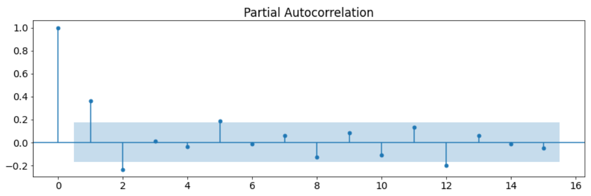
We can use these two methods when deciding on both the correct parameter values and the model suitable for the data. As a result of comparing the two graphs and analyzing the values in these graphs, we can decide which model to use.
The next step is time series estimation methods. The real game starts now :)

What are the time series estimation methods? Let's examine it together!
1) What is autoregressive model (AR Method)?
The autoregressive model is a method based on the assumption that the relationship of the data with the previous data can be explained with a linear model. Explaining the relationship of the data with each other with a linear model is possible with the correlation of the data, in other words, their dependence on each other is high. We learned that the seasonality effect, trend and noise reduce the correlation of the data with each other and change the meaningful properties of the data. For this reason, the auto regression method is used in univariate time series without seasonality, trend and noise.
2) What is Moving Avarage (MA) Method?
The Moving Average (MA) is a forecasting method that acts on the assumption that future data will be close to the average of past data. In this method, we will try to understand the general movement of our series by averaging a certain number of historical data for each data. As the data we process changes, the averaged range will also change. For example, if we are doing our analysis by looking at the previous 2 data, we take the average of the 5th and 6th data while estimating the 7th data. In the next step, we take the average of the 6th and 7th data while processing for the 8th data. Since the averaged range moves, this method is called a moving average. How many data to average will depend on the data and the purpose of the analysis. Predictions made by averaging small intervals will be short term predictions. In order to determine the long-term situation of the data, the larger window interval (lag) should be averaged during the analysis phase.
3) What is Autoregressive Moving Average (ARMA) Method?
Autoregressive Moving Average (ARMA) is a combination of moving average and auto regression techniques. The ARMA method is a technique that aims to predict both future data and future errors simultaneously. While estimating the future values with the auto regression (AR) component of the model, future errors are estimated with the moving average (MA) component. The ARMA model takes two parameters and is represented as ARMA(p,q). The "p" parameter represents how many past data will be considered when estimating future data and is used by the auto regression component. The "q" parameter, on the other hand, represents how many errors in the past will be taken into account when estimating future errors and is used by the moving average component. In other words, the "p" parameter represents the lag number for the data, while the "q" parameter represents the lag number for the error values. For example, let's say we are trying to estimate the 7th data and error with the ARMA(3,2) model. When estimating the data, we use data 4, 5 and 6 and form our estimation. While estimating the error, the error values of the 5th and 6th data are used and the error estimation is created. By evaluating these two estimates together, a more comprehensive analysis result is obtained.
4) What is Autoregressive Integrated Moving Average (ARIMA)?
ARIMA is the ARMA model where the differencing process is applied to make the series stationary. We have examined that the previous data was extracted from each data in the difference taking process and a new series was obtained. We can determine the number of times we will do this process in the ARIMA model. The parameter "d" is also called the degree of difference taking and allows us to specify how many times the difference taking operation will be performed in the series. After this procedure, it is the same as the ARMA model. When predicting the future data in the series obtained as a result of the difference taking process, both data values and error amounts are tried to be estimated. The parameters of the ARIMA model are symbolized as follows.
ARIMA(p, d, q): AR(p) + I(d) + MA(q)
5) What is the Seasonal Autoregressive Integrated Moving Average (SARIMA)?
The Seasonal Autoregressive Integrated Moving Average (SAR Dec) model is an ARIMA model that includes the seasonality component. The SARIMA model includes both the parameters of the ARIMA model and the parameters of the seasonality component. We can symbolize the SARIMA model as follows.
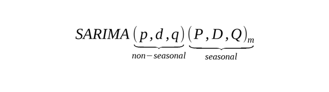
Let's examine the parameters here together!
m parameter: With this parameter, we determine how long it takes for the seasonal cycle in the series to be completed. For example, if the data is monthly and has an annual cycle, the value of m parameter would be 12. The data in this example will show similar behavior in the same month of each year. For example, the movements in January of each year will be similar to each other. Let's examine other seasonality parameters through this example.
P parameter is the parameter by which we can determine how many seasons in the past will be analyzed while estimating the data with Auto Regression (AR). For example, if the parameter P is 3 and we are forcesting for January, we use January data from the previous three years.
D parameter is the parameter that determines the number of times to get the difference. While taking the difference, the January value of the previous season is subtracted from the current data. For example, if the parameter D is 2, we subtract the value of the previous January from the value in January, and we get a new January series. This is the 1st transaction, but our difference was two. When we apply the difference process to the January data we have just obtained, we will reach the result for the month of January. When we apply these operations for other seasons, we make all the data stationary.
Q parameter is the parameter that determines how many error values of the past seasons will be examined when forcesting the error value with the Moving Average (MA). For example, if this value is 4 and we are making an error estimation for the month of January, we use the error values for the January months of the past 4 years.
It should be noted that we made these examples assuming our data had a seasonal cycle of 12 months. If our data had a 4-month cycle, we would use the data from 4 months ago, not 12 months ago as the previous season.
6) What is Vector Auto Regression (VAR) Method?
Vector Auto Regression (VAR) method is the Autoregression (AR) method used for multiple variables (dimensions). The VAR model adopts the same principles as the AR model. The only difference is that the VAR method applies these principles to multivariate models.
7) What is Vector Autoregressive Moving Average (VARMA) Method?
The Vector Autoregressive Moving Average (VARMA) method is the ARMA method used for multiple variables. The principles and methods in the VARMA method are the same as in the ARMA model. The only difference is that the VARMA method is used for multivariate models.
8) How is Time Series Analysis Performed with Machine Learning Techniques?
The basic principle is the same when performing time series analysis with machine learning techniques. We give the data we make stationary as input to machine learning algorithms. These algorithms examine the data according to various statistical principles and learn the structure of the data by analyzing the changes in the data. Machine learning algorithms have different advantages and disadvantages from each other. For this reason, which algorithm to use is important for the result of the analysis.
There are other methods besides these methods in time series, but in general, these are the methods that are most used and give the best results. Now we can examine our future data according to scientific foundations and make our plans according to these results. You can follow my accounts below in order not to miss similar content.
Linkedin: www.linkedin.com/in/mustafabayhan/
Medium: medium.com/@bayhanmustafa
Kaggle : www.kaggle.com/mustafabayhan
We came this far together. Of course, we deserve a celebration.

Tags about Time Series
Time Series forecast Time Series Model Time Series Data Examples
About author

Mustafa Bayhan
Hi, I'm Mustafa Bayhan. I am an Industrial engineer who works in data-related fields such as data analysis, data visualization, reporting and financial analysis. I am working on the analysis and management of data. My dominance over data allows me to develop projects in different sectors. I like to constantly improve myself and share what I have learned. It always makes me happy to meet new ideas and put these ideas into practice. You can visit my about me page for detailed information about me.
You may also like


0 Comments
Leave a Reply
Recent Posts

Kumru AI İncelemesi: Güçlü Yönleri, Zayıf Yönleri ve Kullanım Deneyimi

Large Language Models (LLMs): RAG, Context Engineering, and AI Agents

Model Selection in Data Analysis: What are AIC and BIC?

Types and Meanings of Histograms Used in Data Analysis

Can Correlation Be Used to Infer Causality?
Histogram Nedir, Histogram Grafiği Nasıl Yapılır?