Excel, the leading program in the field of analysis, facilitates operations on data thanks to its numerous formulas and plays a major role in the advancement of analysis studies. Excel allows us to organize, visualize and analyze data with thousands of formulas. Among these thousands of formulas, we will examine together the formulas that are most important for data analysis and most frequently used in projects. Let's get started then!

What are the Most Important Excel Formulas for Data Analysis?

1. What is VLOOKUP Formula?

Vlookup formula is an Excel formula that allows us to search for a certain value in Excel and get results corresponding to this value. For example, in a large table with employees and their birth dates, are you looking for the birth dates of some employees? The vertical drop formula will happily do this job for you.

• How to use the VLOOKUP formula?

How to use the VLOOKUP formula?We can start using the VLOOKUP formula by typing "=VLOOKUP" in Excel. The representation of the VLOOKUP formula with its parameters is as follows.

=VLOOKUP (SEARCH VALUE, FIELD WE WANT TO SEARCH, ORDER NUMBER OF THE TARGET COLUMN, MATCHING STATUS)

We can use the matching status parameter in the formula by typing 1 or 0. When we want to find the exact value we are looking for, we must write 0 to this parameter. If it is enough for us that the value we are looking for is approximately similar, we should write 1 to this parameter. For more detailed information about the VLOOKUP formula, you can read my post titled as What is the Vlookup Formula?

2. What is the IFS Formula?

IFS formula is an excel formula that allows us to test multiple conditions simultaneously. When there is more than one condition, the nested IF formula can also be used, but choosing the IFS formula instead would be a more efficient method. To access the multivalue formula, it is sufficient to type =IFS in Excel. In the multi-if formula, the conditions and the action to be taken if the condition is met are written respectively. Excel checks the conditions one by one, starting from the first condition, and performs the action for that condition if it occurs. For example, imagine that you are a professor calculating students' letter grades. Wouldn't you like to effortlessly calculate letter grades with a single formula? That formula is the IFS formula. For more detailed information about the IFS formula, you can read my post titled as What is the IFS Formula?

• How to use the IFS formula?

The usage of the IFS formula along with its parameters is as follows.

=IFS(condition1,process1,condition2,process2, … ,condition127,process127)

We can write an example of the IFS formula that calculates letters according to student grades as follows. In this example, we used a condition called TRUE. Our goal here is to determine what to do in the remaining situations if the previous conditions are not met.

=IFS(B2>89;“A”;B2>79;“B”,B2>69;“C”;B2>59;“D”;TRUE,“F”)

3. What is SUMIFS formula?

The SUMIF formula is an excel formula that allows us to filter data by certain conditions in one go and sum the values that meet our conditions. For example, a research is being conducted on female employees in the company who know Excel. Let's say we're trying to total the salaries of these employees. In this example we have two conditions. She will be a working woman and will know how to excel. We can easily collect the salaries of employees who meet these conditions using the add-together formula.

• How to use the SUMIFS formula?

The usage of the sumifs formula along with its parameters is as follows.

=SUMIFS(range_total; criteria_range1; criteria1; criteria_range2; criteria2) 

We start the process by specifying which column we will sum. In our example, we must select the salary column since we will be collecting salary values. Then, we write the conditions we want to occur into the formula. In our example regarding employees, we can achieve the result we want by creating a formula as follows.

=SUMIFS(D2:D6;C2:C6;"Knows";B2:B6;"Woman")

4. What is CONCAT Formula?

Concat formula is an excel formula that allows us to combine cells and text strings in excel. The concat formula, which is very simple to use, is an important formula preferred in many projects. To use the concat formula, we just need to write the cells and text strings we want to merge into the formula. The Concat formula will do that magic and give us these values combined.

• How to use CONCAT formula?

We can use the concat formula using the following syntax.

=CONCAT(text1; [text2], …)

The following operation, in which we combine two columns and put a dash between them, is an example of using the CONCAT formula.

5. What is REPLACE formula?

When using the Replace formula, we first write the text string or cell we will edit into the formula. Afterwards, we write down from which character we want to change. The next parameter is how many characters we want to change. Finally, we add to the REPLACE formula what the characters we selected will be replaced with. The syntax of the Replace formula is as follows.

• How to use the Replace formula?

When using the Replace formula, we first write the text string or cell we will edit into the formula. Afterwards, we write the number of characters we want to change, starting from the last character, into the CHANGE formula. Finally, we add to the formula what the characters we selected will be replaced with. The syntax of the Replace formula is as follows.

=REPLACE(old_text; start_num; end_num; new_text)

In the following example, we have edited the 3 commas in the middle using the REPLACE formula and replaced the commas with the value "456".

6. What is UNIQUE formule?

Unique formula is an excel formula that allows removing duplicates in a range. As a result of this formula, we obtain a new list in which each value is included once.

• How to use the unique formula?

Unique formula is one of the easiest formulas to use. To use the formula, it will be sufficient to write a range in the formula. We can use the unique formula with the following syntax.

=UNIQUE(array, [by_col], [exactly_once])

Unique formula has 3 parameters. We start the process by specifying the range in the first parameter. We can also use the formula only this parameter. The other two parameters are optional parameters.

With the "by_col" parameter we determine whether the unique formula looks at columns or rows. By default, this parameter is set to check rows. If we write TRUE to this parameter, we make the columns unique, and if we write FALSE, we make the rows unique.

If we write TRUE to the "exactly_once" parameter, the formula will bring the values that occur only once to the new list. If any data is repeated, the formula will delete this data and not add it to the new list.

Let's make examples of its UNIQUE formula then!

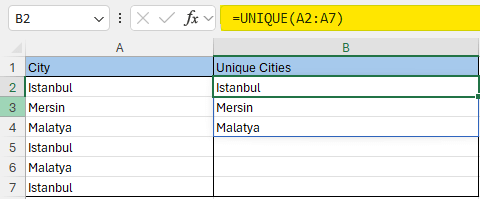
In the Unique formula example below, there are city names in the City column and some cities are repeated. When we look at the second column, we reach the unique state of the cities. Since the cities of Istanbul, Mersin and Malatya were located in the first column, its unique formula brought these values to the second column.

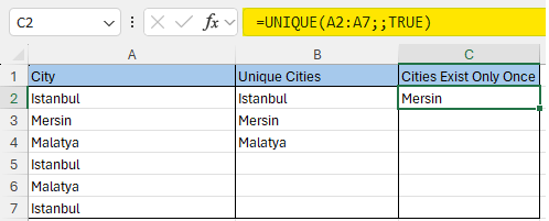
Let's examine the exact_once parameter, which is the third parameter of unique formula, with the same example. By typing TRUE in this parameter, we will access the data that appears only once in the first column. Let's try it and see the difference together!

As seen in the picture above, the only data in the first column that did not repeat and was found once was the city of Mersin. We set the exactly_once parameter in the unique formula to TRUE and obtained non-repetitive data.

7. What is IFERROR Formula?

The iferror formula is an Excel formula that allows us to take extra action where errors will occur. With the if-error formula, we can intervene in places where we do not want to receive errors, and at the same time, we can determine how our project will behave in case of errors we receive. The if-error formula is among the most important formulas in Excel, as it both prevents unexpected results in projects and increases the efficiency of work.

• How to use the iferror formula?

Iferror formula is very easy to use and integrate into our projects. The first thing we need to do is to write the operation or cell that is likely to cause an error into the formula as the first parameter. The second parameter of the iferror formula is the action to be taken in case of an error. When an error occurs, the operation in the second parameter is activated and the operation we want to be performed in case of error is performed. The iferror formula, which works with these two parameters, increases the efficiency of our projects and also makes the projects easier to use. Let's do an example using the iferror formula!

When a number is divided by 0, the #DIV/0! error occurs like in cell C2. We used the iferror formula to avoid this error. We both prevented errors from occurring and printed text in the cell in case an error occurred.

Abstract

Excel, one of the leading programs in data analysis, is frequently preferred in analysis studies due to its many functional formulas and its ability to remain up-to-date. We examined the important formulas preferred in data analysis of Excel, which will maintain its advantage for a long time because it makes things easier. We can make our projects more functional and efficient by using these formulas in our future work.

If you would like to be informed about developments and sample studies regarding Excel and Excel formulas, you can follow me on the accounts below.

Linkedin: www.linkedin.com/in/mustafabayhan/

Medium: medium.com/@bayhanmustafa